Showcase · Data layers · City of Melbourne and Victorian open data

One school record. Thirteen buildings.

What does one shape per school hide? One school drawn as its buildings, rolled up to the site, with estimated floor space per student.

The other school maps draw one shape per school and divide its grounds (the land a school sits on, buildings included) by its students. That is a site-level figure. Here one campus, University High School in Parkville, is drawn as its buildings, each its own shape with its own data, then rolled back up to the site. One shape says 24,233 m² of grounds for 1,983 students in 2025: 12.2 m² each. The students figure is the February FTE enrolment (Victorian Department of Education), not a headcount. The council’s land use census has one record for the school: built 1930, 3 floors. Its 2023 footprints show 13 buildings.

One shape per school hides the buildings

A school map that keys one shape to one school can give each student’s share of the grounds. It cannot say how much floor space there is, which buildings are old, which are temporary, or which a wheelchair user can get into. The council’s Census of Land Use and Employment (CLUE) records buildings, but for this property it has one record: University High School, built 1930, refurbished 2008, 3 floors, accessibility rated moderate. The science school next door, the school’s branch for Years 11 and 12, has its own: built 2014, 3 floors, rated high. The other 11 buildings have no record at all.

The map

Switch between the site as one shape and its buildings, coloured by era, by storeys or by their share of the floor. Hover over a building, or tap it on a phone, for its numbers.

Grounds are not floor space

The Sydney schools showcase measures grounds per student, one shape per school. Building by building, Plotlay can answer the other question. Each building’s height comes from the council’s 3D footprints; its storeys are estimated from that height (or taken from the census where it has a record), and its floor space from the storeys over its footprint. Rolled up to the site, the 13 buildings have an estimated 23,624 m² of floor space, 2.49 times their 9,484 m² footprint: about 11.9 m² of floor space (estimated) per student in 2025, against 12.2 m² of grounds. Enrolments are the school’s, so they are divided at site level only, never split across buildings.

More students, the same grounds

February enrolments rose from 1,210 in 2007 to 1,990 in 2026, on the same 24,233 m². Grounds per student fell from 20.0 m² to 12.2 m². The council’s footprint snapshots show where the room came from: six single-storey buildings of 195 to 205 m² each, 3.7 to 4.0 m high with gable roofs, are not on the 2020 footprints and are on the 2023 ones (captured January 2022). Together they add 1,195 m², 5.0% of the campus’s floor space. Enrolment grew by 321 between 2020 and 2025.

Sample data

Running the campus: facilities on the same buildings

The real analysis ends above. Once each building is a keyed shape, a facilities team can hang everything it runs on them: the asset register, risk, work orders, planned maintenance, essential safety measures, the asbestos register, meters and the capital plan. This section shows that for the same 13 buildings, using sample data: the figures are not about University High School or any real building.

Sample data226assets in the register, each a point inside its building

Sample data40at high or extreme risk (likelihood x consequence)

Sample data36work orders open, 17 past their target

Sample data86.9%of planned maintenance done on time over the year

Sample data7 of 50essential safety measures overdue

Sample dataA$3.9Mof capital works waiting, A$106k due within a year

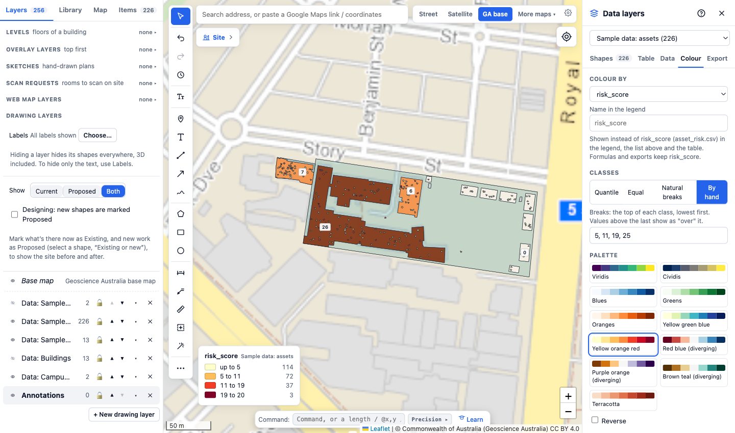
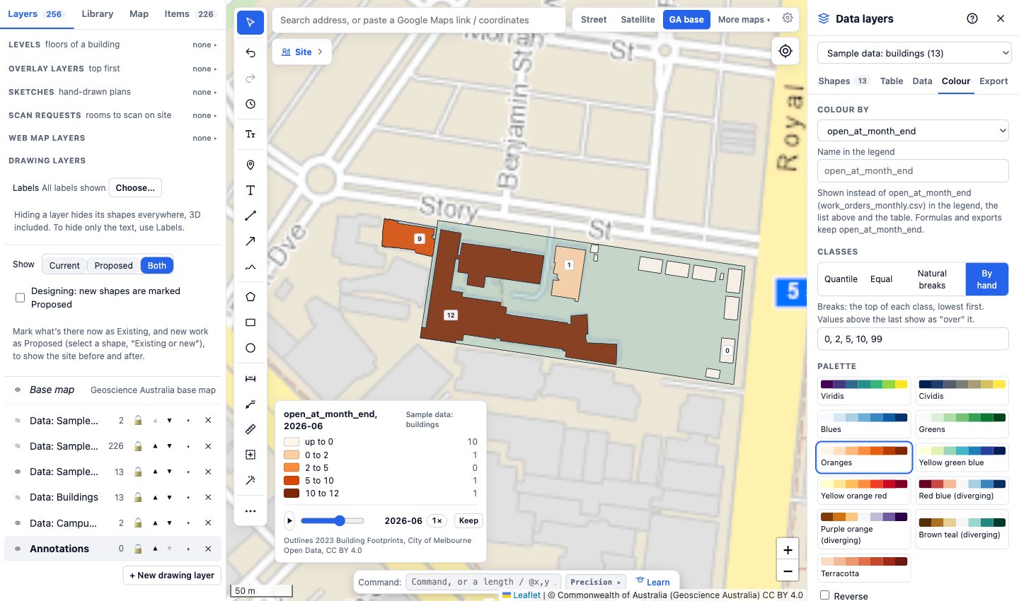
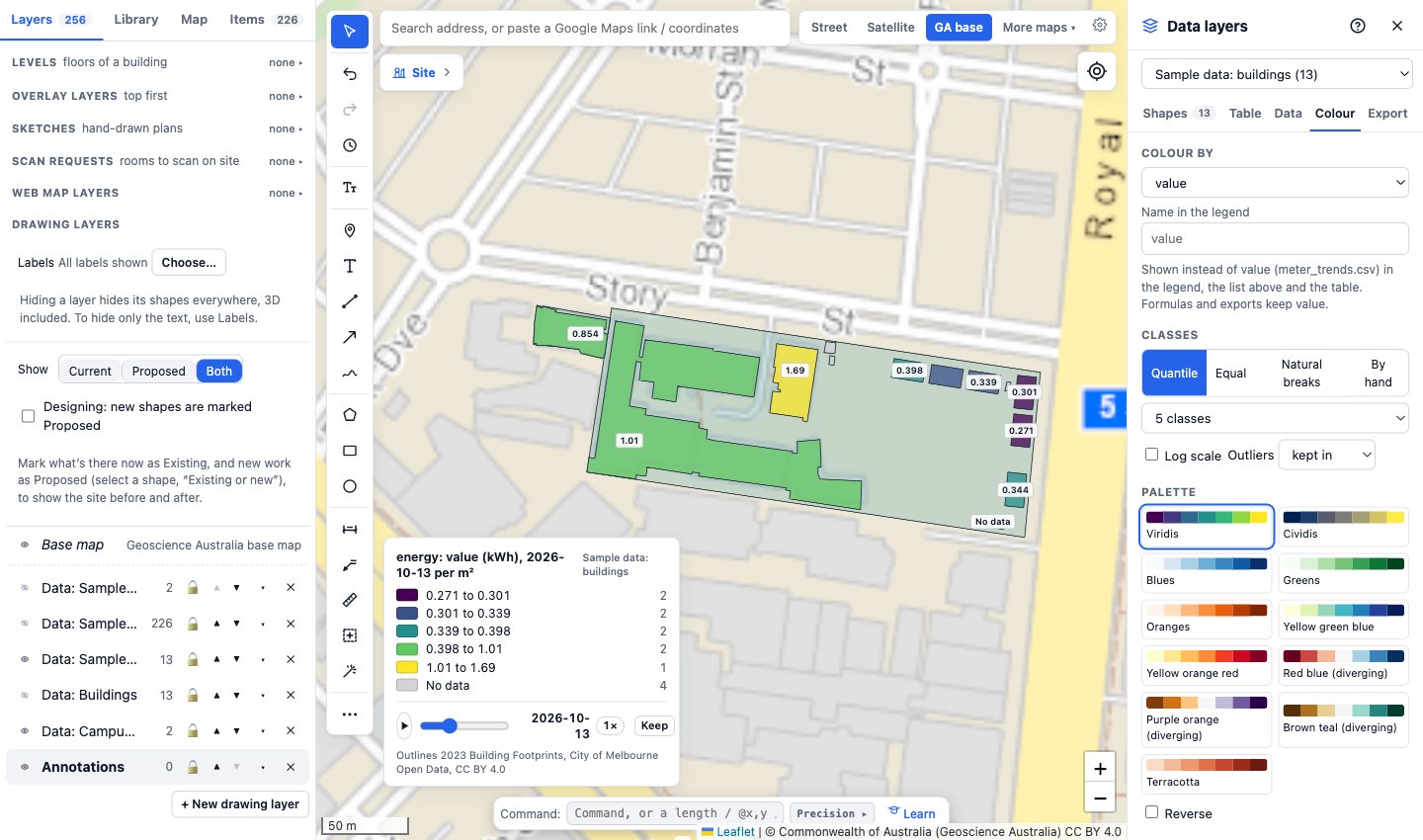
Switch the map between risk, open work orders month by month, the condition of each building, its share of the capital backlog and the power it uses after hours. In the risk view every asset is a dot: hover or tap one for its tag, condition, life left and next service.

RiskWork ordersConditionBacklogAfter-hours power

Where the risk sits

Each asset is scored for the likelihood it fails (its condition, its remaining life, whether its service is overdue) and the consequence if it does (a fire panel or a lift more than a split system). 40 of 226 rate high or extreme. Plotlay rolls the assets up into the buildings they stand in, so the map can colour a building by the risk inside it, and rolls the buildings up to the site.

The work order backlog

802 work orders over twelve months: 42% reactive from the helpdesk, the rest routine services raised from the maintenance schedule. 36 are open, 17 past their target. On the map, the work order view steps through the months with the slider.

Is the maintenance being done?

Planned maintenance done by its due date, month by month, and each building’s essential safety measures: current, due within 30 days or overdue, the items an annual essential safety measures report has to account for.

Meters from the BMS

A trend log as a building management system exports it (timestamp, point, value, unit) of every building’s electricity meter, by the hour for four weeks of term. Plotlay’s BMS import reads each point name, B02-EM-01.kWh, and puts it on that building: no rooms needed. The heat map shows B01 and B03 following the school day and B02 using 62% of its power after hours.

The capital plan

Renewals for high-risk assets near the end of their life, roofs, windows and finishes by condition, asbestos removal and accessibility, each project linked to the assets or register items it renews: A$3.9M in all.

How it was done in Plotlay

1. The asset register. 226 assets of Plotlay’s facilities types (switchboards, fire panels, extinguishers, hydrants, lifts, air handling units, roof anchors...) imported with their tags, each a point inside its building, with an inspection form for each type. Six inspections recorded on the forms; the three fails raised corrective actions.
2. Assets as a data layer, keyed by tag with the register’s columns, the risk table linked by asset id and coloured by risk score. The register’s pins can come off the map so the layer reads cleanly.
3. Roll-ups from the assets into the buildings (how many, how many at high risk, the highest score) and from the buildings to the site (assets, open work orders, the backlog).
4. Work orders over time: each building’s open work orders at each month’s end, linked as a time series, so the slider steps through the year.
5. BMS data onto the buildings: the meters’ trend log imported onto the buildings layer by key, then a heat map of power per m².
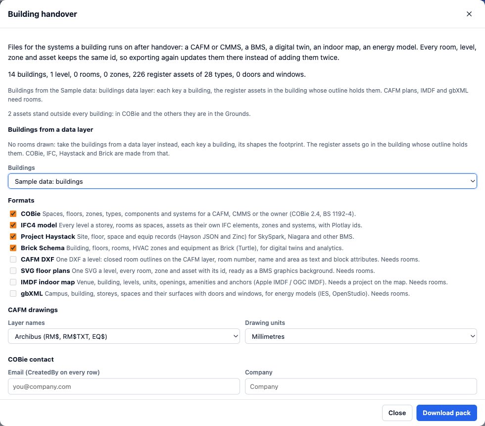
6. Building handover from the buildings layer, with no rooms drawn: COBie, IFC, Project Haystack and Brick, every building and asset with an id that stays the same at the next export.
7. Exports for Power BI (TopoJSON for the Shape Map, CSV with WKT) and Python, as for the real layers.

The sample tables

Eleven tables in the shape a CAFM or CMMS exports, all keyed to the buildings and most to an asset tag, drawn from one fixed seed so anyone can make them again. Columns and how each was drawn are in the data dictionary, data/sample/README.md in the plotlay-school-campus repository.

Table	Rows
assets.csv the asset register: points inside the buildings, Plotlay asset types and tags, condition, life left, next service	226
asset_risk.csv likelihood and consequence per asset, the rating, what drives it and the treatment	226
work_orders.csv 12 months of reactive and planned work orders: trade, priority, status, target, age, cost	802
work_orders_monthly.csv each building at each month’s end: raised, completed, open, overdue	156
pm_compliance.csv planned maintenance by building and month: on time, late, missed	80
esm_register.csv essential safety measures by building: inspections, status, open defects	50
asbestos_register.csv presumed and sampled materials in the older buildings, risk and action	11
meter_trends.csv a BMS trend log: hourly kWh per building meter and kL per water meter, four weeks	8,064
space_use.csv teaching spaces: seats, timetabled periods, frequency, occupancy	16
capital_works.csv the capital works backlog: element, driver, priority, year, estimate	28
building_summary.csv one row per building: everything above rolled up	13

How it was made in Plotlay

1. A map project on the Geoscience Australia base map, and two data layers: Campus site and Buildings (Data layers, in the Site workspace).
2. Start from the data. The enrolments linked to the empty Campus site layer, the 13-row buildings table linked to the empty Buildings layer: every row is one to place.
3. Pick from a layer. The council’s property boundaries (parts joined by property_id) and 2023 building footprints (parts joined by structure_id), with their licence. A click takes the outline under it and gives it the row’s key; the two parcels become parts of one site.
4. A time axis: each building’s footprint on the council’s 2014, 2015, 2018, 2020 and 2023 layers. The slider shows the buildings arrive.
5. Colour by era, by estimated storeys, and by floor space divided by footprint.
6. 3D at the real heights: each building at its council height in metres, in floor plates from its storeys.
7. Roll up the buildings to the site: how many, their footprint, their floor space, the earliest first shown. Formulas give grounds and floor space per student at site level.
8. Sample data on copies of the outlines, in layers of their own (see the facilities section above), and export GeoJSON, TopoJSON for the Power BI Shape Map, CSV with WKT, the linked data and a Python starter.

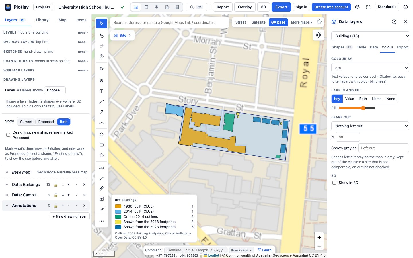
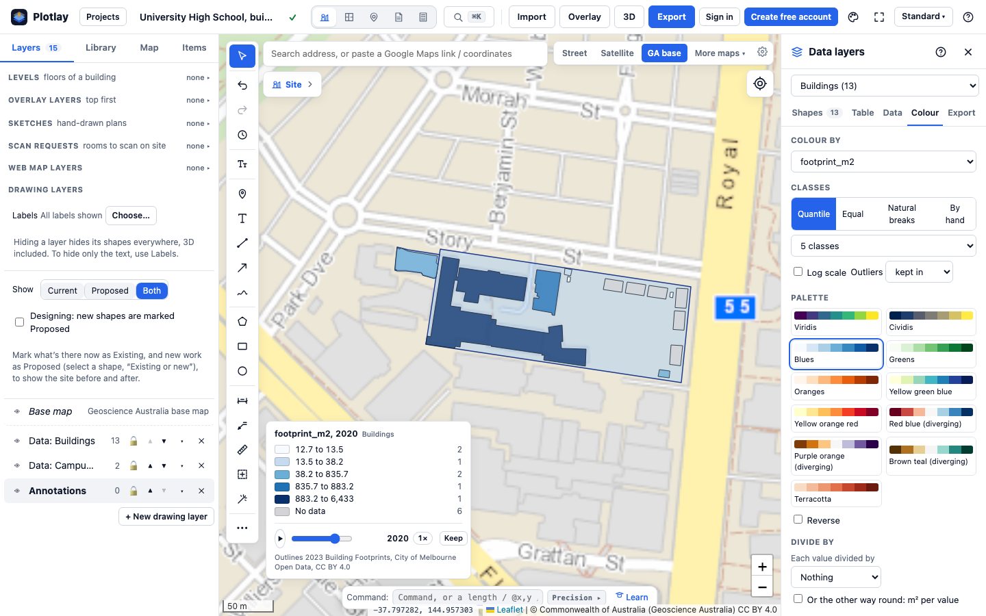
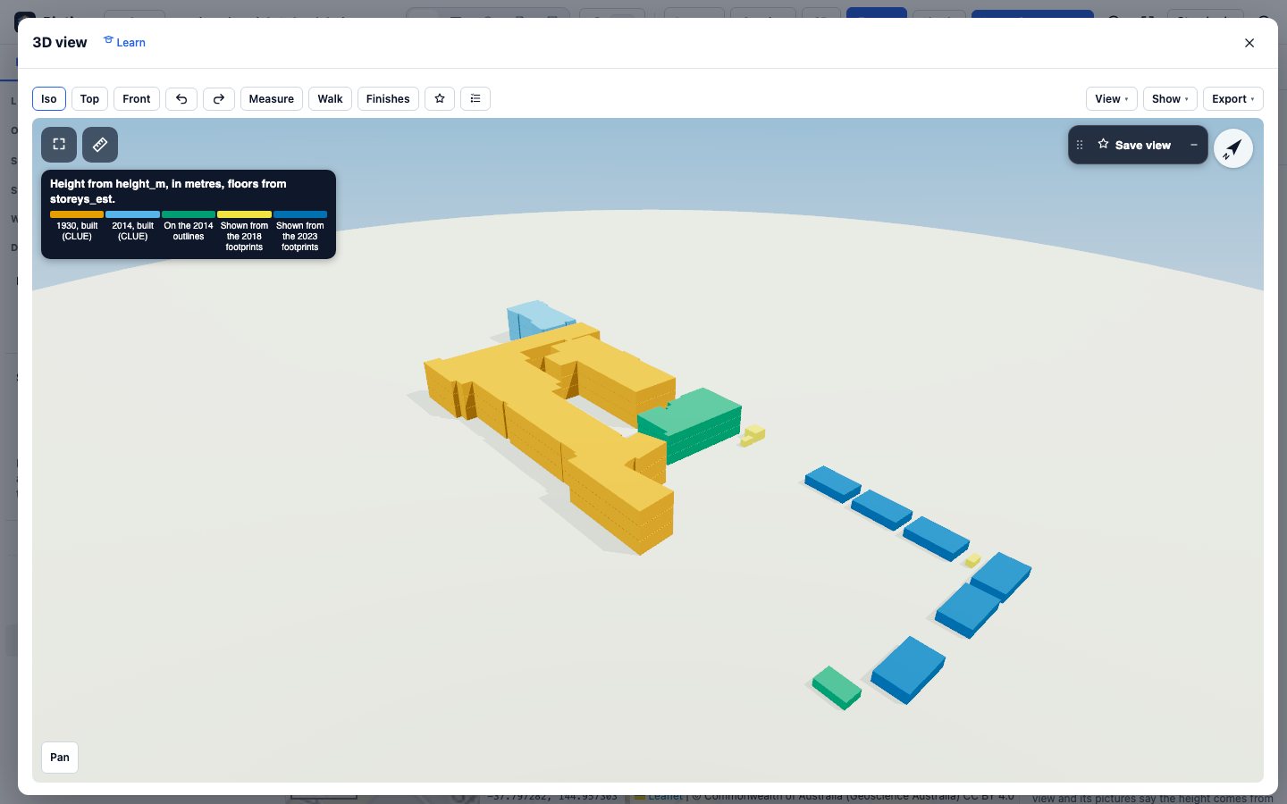
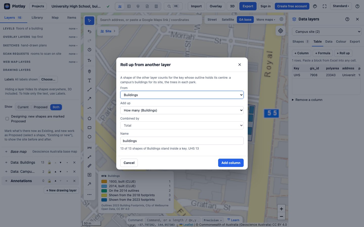
Every building’s area matches the council footprint to within 0.148%.

More about Data layers · Make a data layer of your own

Power BI

The same shapes and tables as a Power BI Project (.pbip): a Shape Map of the buildings from the TopoJSON keyed B01 to B13, site-level measures (grounds, footprint and floor space per student) that never split enrolments across buildings, the footprint on each council snapshot, and three pages of sample data (the risk matrix, the work order backlog, compliance), each tagged Sample data, with the Plotlay theme. It reads the data from the GitHub repository, so it refreshes with no gateway.

The Power BI project is in the plotlay-school-campus repository on GitHub, with the steps to open it in Power BI Desktop.

Python

A narrated Jupyter notebook loads the shapes with GeoPandas, joins the buildings table, checks Plotlay’s roll-up and works out every number on this page. The sample tables are read only in their own section at the end.

Download the notebook (with its outputs) and the data. Both are also in the plotlay-school-campus repository on GitHub.

Read it carefully

• Floor space is an estimate: at each square metre, the council’s height (2 m less under a pitched roof) divided by 4 m floor to floor, rounded, at least one storey, and never more than the census floors where it has a record for the building. A scale and a ranking, not a measured floor area.
• Heights are the council’s: the top of a building’s highest part above the lowest base of the structure. On a sloping site the uphill side reads a little taller.
• Era is a year built for two buildings (the census). For the rest it is the first council layer that shows them; an early layer can leave out a small structure, so first shown is not built.
• Students are the school’s February FTE enrolments (Victorian Department of Education), not a headcount, the science school’s students included. They are divided at site level only.
• Areas are approximate: accuracy depends on the council’s footprints and property boundaries the outlines came from.

The other campus and schools showcases

• A campus drawn out, building by building: TAFE NSW Richmond, where the buildings were in no open map data, drawn out over NSW aerial imagery with each outline’s source and accuracy, then the same facilities section in sample data.
• Sydney schools: grounds per student across 81 inner Sydney and Parramatta government schools (2025 headcount), one shape per school.
• NSW and SA schools side by side: the same grounds method within 7 km of the Sydney and Adelaide town halls (2024 headcount), plus spending, staffing and outcomes for each state.
• Inner Sydney High, a deep dive: a 14-storey vertical school, measured by its estimated floor space per student over its staged opening.