
Showcase · Drawing · Data layers · Facilities · NSW open data
One building on the map. Thirty-eight on the campus.
What if a campus’s buildings are in no map data at all? Draw them out over open aerial imagery, record where each outline came from and how accurate it is, then key the asset register, work orders and capital plan to each one.
TAFE NSW Richmond sits on 32 ha of the Hawkesbury flood plain. OpenStreetMap has 1 building inside it. NSW’s building footprint layer is not open. The land title is a 292 ha lot shared with the university next door, so there is no parcel to start from either. Microsoft’s building outlines, made by software from aerial photos, find 33 shapes, rough and a metre or three off. Plotlay draws out all 38 buildings over NSW aerial imagery, and each one carries where its outline came from and how far it can be trusted.

The map data has one building
Most asset work starts from a footprint someone else drew. Here there is almost nothing to start from. OpenStreetMap shows 1 building inside the campus. The state’s footprints are licensed to government agencies only. The cadastre lot is 292 ha and holds the university’s campus too. The best open outlines are Microsoft’s building outlines, made by software from aerial photos: 33 shapes, which miss 5 buildings and sit a median 2.23 m off the roofs they describe.
The map
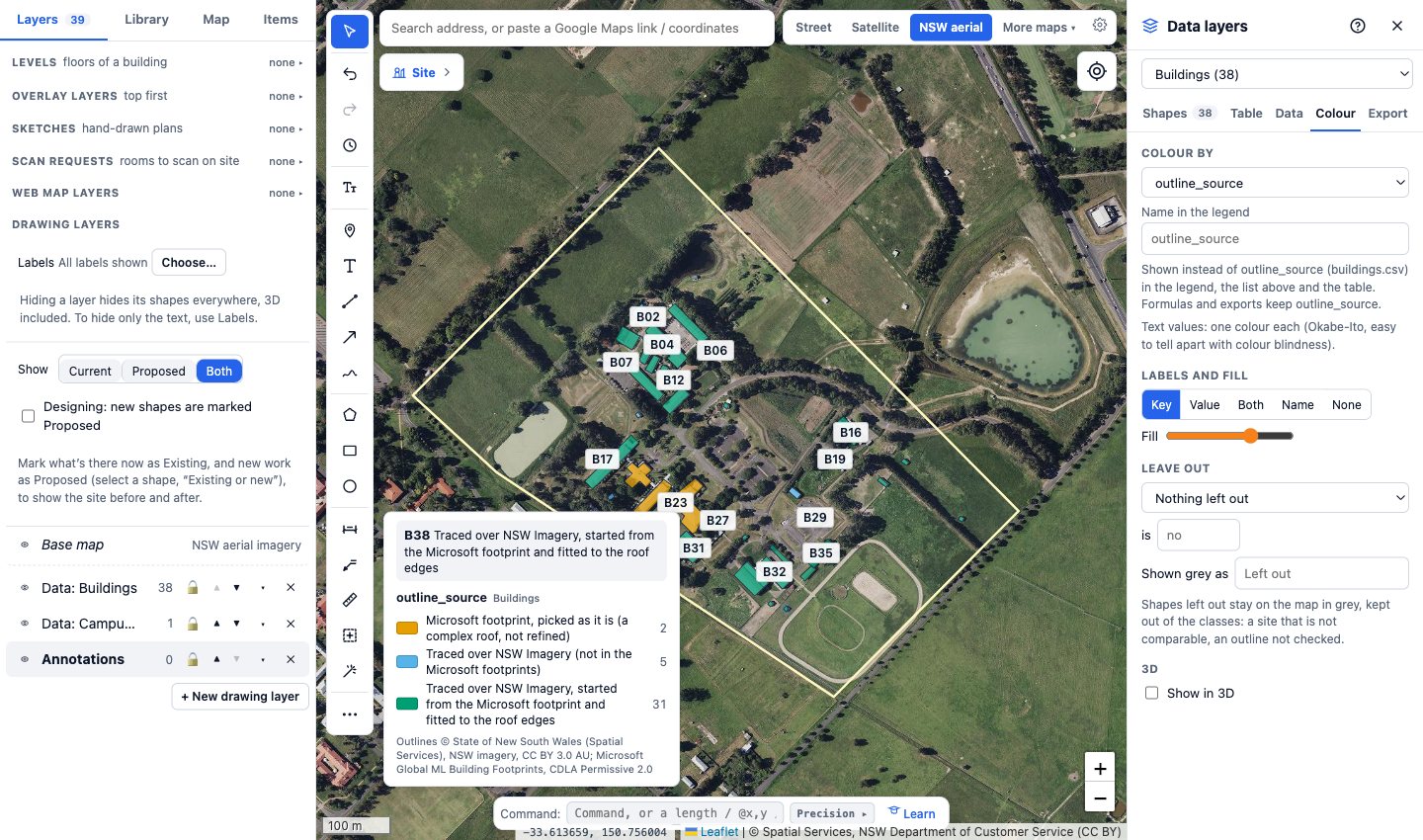
Each building over the imagery, coloured by where its outline came from, by how far Microsoft’s outline was off, or by its size. Hover over a building, or tap it, for its source and accuracy.
Drawing them out
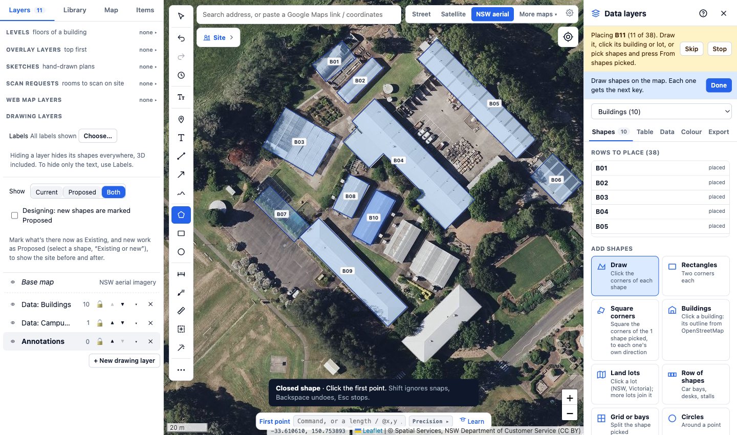
The imagery is NSW Spatial Services’ aerial photography, licensed CC BY 3.0 AU, sharp enough at this site to see roof sheets (about 7 cm a pixel). In Plotlay, on the NSW aerial imagery base map, each building is drawn corner by corner on a data layer. Where Microsoft’s outline was usable it was the starting point and the corners went onto the roof edges; where there was nothing, the building was drawn from scratch. Square corners as I draw squares each outline to its own direction (the campus grid runs about 42° off east). Two buildings with complex roofs, a cross and joined wings, were picked from Microsoft’s footprints as they are, to show snapping to what exists, and are marked less accurate. Every shape keeps its source: drawn over NSW aerial imagery, or picked from a file with its licence.
| Outline source | Buildings | Accuracy |
|---|---|---|
| Traced over NSW Imagery (not in the Microsoft footprints) | 5 | ±0.5 m |
| Traced over NSW Imagery, started from the Microsoft footprint and fitted to the roof edges | 31 | ±0.5 m |
| Microsoft footprint, picked as it is (a complex roof, not refined) | 2 | ±2.5 m |
Accuracy depends on the imagery: a roof outline includes the eaves, so a wall line sits a little inside it, and a shadow or a tree over an edge can hide it. The accuracy column is what the drawing method can hold to; where law or a contract needs a licensed surveyor, their licence and sign-off are what count.


Asset outcomes, building by building
With every building a keyed shape, the asset register, work orders, maintenance, compliance and the capital plan can be linked to it. This section shows that for the same 38 buildings, using sample data: the figures are not about TAFE NSW Richmond or any real building.
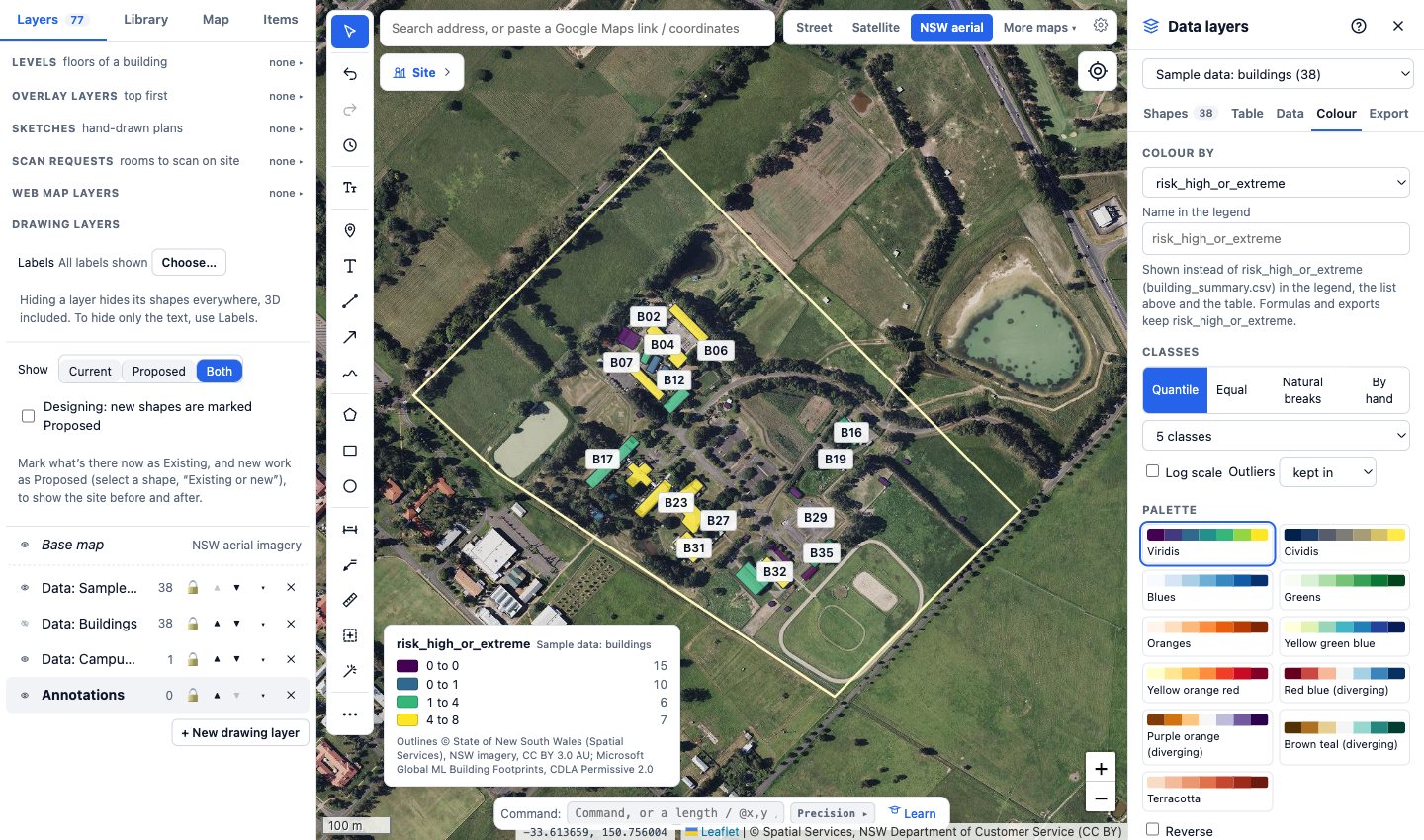
Switch the map between risk, open work orders month by month, condition, backlog and power used after hours. In the risk view every asset is a dot: hover or tap one for its tag, condition, life left and next service.


The sample tables
Eleven tables in the shape a CAFM or CMMS exports, keyed to the buildings and most to an asset tag, drawn from one fixed seed with the same generator as the University High School showcase (its own seed, its building plan made by rules from the footprints). Columns and how each was drawn are in the data dictionary, data/sample/README.md in the plotlay-tafe-richmond repository.
| Table | Rows |
|---|---|
assets.csv the asset register: points inside the buildings, Plotlay asset types and tags, condition, life left, next service | 372 |
asset_risk.csv likelihood and consequence per asset, the rating, what drives it and the treatment | 372 |
work_orders.csv 12 months of reactive and planned work orders: trade, priority, status, target, age, cost | 1,010 |
work_orders_monthly.csv each building at each month’s end: raised, completed, open, overdue | 456 |
pm_compliance.csv planned maintenance by building and month: on time, late, missed | 257 |
esm_register.csv essential safety measures by building: inspections, status, open defects | 131 |
asbestos_register.csv presumed and sampled materials in the older buildings, risk and action | 20 |
meter_trends.csv a BMS trend log: hourly kWh per building meter and kL per water meter, four weeks | 16,800 |
space_use.csv teaching spaces: seats, timetabled periods, frequency, occupancy | 19 |
capital_works.csv the capital works backlog: element, driver, priority, year, estimate | 82 |
building_summary.csv one row per building: everything above rolled up | 38 |
How it was made in Plotlay
- A map project on NSW aerial imagery (in the base map list under Government (AU)), allowed in exports.
- Campus site: a one-row table linked to an empty data layer, its key placed by drawing the campus along its fences and roads.
- Buildings: the 38-row table linked, then Place them one by one: each row drawn corner by corner with Square corners as I draw on, or picked from Microsoft’s footprints added with their licence. Each shape keeps its source.
- Colour by outline source and by how far Microsoft’s outline was off.
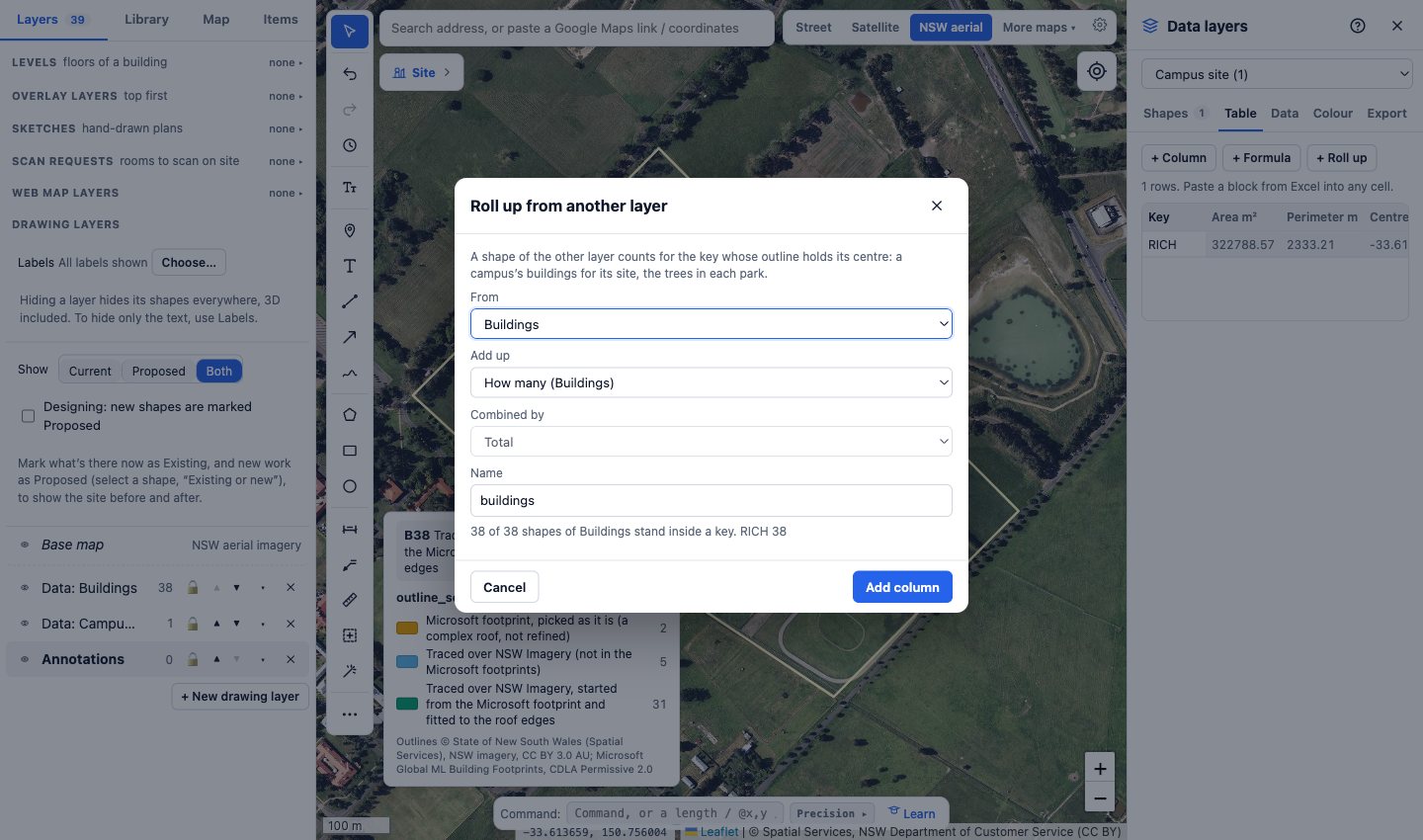
- Roll up the buildings to the site: how many, their footprint.
- Sample data: the register’s assets as points keyed by tag, rolled up into the buildings and the site; work orders by month on the time slider; the meters’ trend log imported onto the buildings by key; the building handover pack (COBie, IFC, Haystack, Brick) from the buildings layer, with no rooms drawn.
- Charts and map pictures from Plotlay’s own chart engine (Analysis), and exports for Power BI and Python.
More about Data layers · Make a data layer of your own
Power BI


The same shapes and tables as a Power BI Project (.pbip): a Shape Map of the buildings from the TopoJSON keyed B01 to B38, the outline sources and accuracy, and three pages of sample data (risk, work orders, compliance), each tagged Sample data, with the Plotlay theme. It reads the data from the GitHub repository, so it refreshes with no gateway. It is in the plotlay-tafe-richmond repository on GitHub, with the steps to open it.
Python
A narrated Jupyter notebook loads the shapes with GeoPandas, checks the outline sources and accuracy against the drawing, compares Microsoft’s footprints, checks Plotlay’s roll-up and reads the sample tables in their own section.
Download the notebook (with its outputs) and the data. Both are also in the plotlay-tafe-richmond repository on GitHub.
Read it carefully
- Areas and outlines are approximate: accuracy depends on the imagery they were drawn over and on how each was drawn (the table above). A roof outline includes the eaves.
- The campus outline follows the fences and roads seen in the imagery, not a title boundary: the land title is a 292 ha lot shared with the university.
- Building uses, heights and storeys are not recorded here; the sample treats every building as one storey.
- Everything in the facilities section is sample data, generated for this page from the building sizes alone.
The other campus and schools showcases
- One school campus, building by building: University High School, Parkville, where the buildings were already in the council’s footprints, rolled up to the site, with the same facilities section in sample data.
- Sydney schools: grounds per student across 81 inner Sydney and Parramatta government schools, one shape per school.
- Inner Sydney High, a deep dive: a 14-storey vertical school, measured by its floor space (estimated) per student.
Sources and licences
Aerial imagery, and the outlines drawn over it: © State of New South Wales (Spatial Services, a business unit of the Department of Customer Service NSW), licensed under CC BY 3.0 AU. Building outlines drawn over NSW Imagery in Plotlay. Two outlines, and the starting points of others: Microsoft Global ML Building Footprints, CDLA Permissive 2.0. The facilities figures are sample data.
Base maps on this page’s maps: NSW Imagery © State of New South Wales (Spatial Services), CC BY 3.0 AU (the campus map); © Commonwealth of Australia (Geoscience Australia), CC BY 4.0 (the facilities map). Maps: Leaflet.
Our shapes and tables are CC BY 4.0 and the code is MIT. This is independent work using open data, not endorsed by TAFE NSW or Spatial Services.
Draw out your own campus
Plotlay is free to start: every tool, three cloud projects.
Create free accountThen open Data layers in any map project